Data Source : https://www.rbnz.govt.nz/statistics/series/economic-indicators/prices
New Zealand Inflation – Time Series Analysis
Chandan Kumar
1. Setup & Libraries
library(tidyverse)
library(forecast)
library(tseries)
library(zoo)
library(lubridate)
library(gridExtra)
library(knitr)
library(scales)
2. Data Loading & Cleaning
The CSV has two header rows (category names + metric sub-labels). We skip both and assign clean column names manually.
# Read raw without headers
raw <- read.csv("Prices-Inflation.csv", header = FALSE, stringsAsFactors = FALSE,
                na.strings = c("", "NA"))

# Row 1 = category names, Row 2 = sub-metric labels, Row 3+ = data
col_names <- c(
  "Date",
  "CPI_Index", "CPI_qq", "CPI_yy",
  "Tradable_Index", "Tradable_qq", "Tradable_yy",
  "NonTradable_Index", "NonTradable_qq", "NonTradable_yy",
  "Food_Index", "Food_qq", "Food_yy",
  "Housing_Index", "Housing_qq", "Housing_yy",
  "Transport_Index", "Transport_qq", "Transport_yy",
  "Petrol_Index", "Petrol_qq", "Petrol_yy",
  "CPI_ExPetrol_Index", "CPI_ExPetrol_qq", "CPI_ExPetrol_yy",
  "TrimmedMean_qq", "TrimmedMean_yy",
  "WeightedMedian_qq", "WeightedMedian_yy",
  "FactorModel_yy",
  "SectoralFactor_yy", "SectoralTradable_yy", "SectoralNonTradable_yy",
  "HPI_Index", "HPI_qq", "HPI_yy",
  "GDPDeflator_Index", "GDPDeflator_qq", "GDPDeflator_yy",
  "PPI_Input_Index", "PPI_Input_qq", "PPI_Input_yy",
  "PPI_Output_Index", "PPI_Output_qq", "PPI_Output_yy"
)

df <- raw[3:nrow(raw), 1:length(col_names)]
colnames(df) <- col_names

# Parse date and numeric columns
df <- df %>%
  mutate(Date = as.yearqtr(Date, format = "%b %Y")) %>%
  mutate(across(-Date, ~ suppressWarnings(as.numeric(.x)))) %>%
  arrange(Date) %>%
  filter(!is.na(CPI_Index))

cat("Data range:", format(min(df$Date)), "to", format(max(df$Date)), "\n")
## Data range: 1988 Q1 to 2026 Q1## Rows: 153 | Columns: 45| Date | CPI_Index | CPI_qq | CPI_yy | Tradable_Index | Tradable_qq | Tradable_yy | |
|---|---|---|---|---|---|---|---|
| 146 | 2024 Q2 | 1272 | 0.4 | 3.3 | 1184 | -0.5 | 0.3 |
| 147 | 2024 Q3 | 1280 | 0.6 | 2.2 | 1182 | -0.2 | -1.6 |
| 148 | 2024 Q4 | 1287 | 0.5 | 2.2 | 1185 | 0.3 | -1.1 |
| 149 | 2025 Q1 | 1299 | 0.9 | 2.5 | 1194 | 0.8 | 0.3 |
| 150 | 2025 Q2 | 1306 | 0.5 | 2.7 | 1198 | 0.3 | 1.2 |
| 151 | 2025 Q3 | 1319 | 1.0 | 3.0 | 1208 | 0.8 | 2.2 |
| 152 | 2025 Q4 | 1327 | 0.6 | 3.1 | 1216 | 0.7 | 2.6 |
| 153 | 2026 Q1 | 1339 | 0.9 | 3.1 | 1224 | 0.7 | 2.5 |
3. Exploratory Data Analysis
3.1 Headline CPI – Level & Annual Change
p1 <- ggplot(df, aes(x = as.Date(Date), y = CPI_Index)) +
  geom_line(color = "#2c7bb6", linewidth = 0.9) +
  labs(title = "Headline CPI Index (Base ~1000)", x = NULL, y = "Index") +
  theme_minimal(base_size = 13)

p2 <- ggplot(df %>% filter(!is.na(CPI_yy)), aes(x = as.Date(Date), y = CPI_yy)) +
  geom_line(color = "#d7191c", linewidth = 0.9) +
  geom_hline(yintercept = c(1, 3), linetype = "dashed", color = "grey50") +
  annotate("rect", xmin = as.Date("1988-01-01"), xmax = as.Date("2026-12-31"),
           ymin = 1, ymax = 3, alpha = 0.08, fill = "green") +
  labs(title = "CPI Annual Inflation (y/y %)", x = NULL, y = "y/y %",
       caption = "Green band = RBNZ 1–3% target range") +
  theme_minimal(base_size = 13)

grid.arrange(p1, p2, ncol = 1)
3.2 All Key Series – Annual Inflation
yy_long <- df %>%
  select(Date, CPI_yy, Tradable_yy, NonTradable_yy, Food_yy,
         Housing_yy, Transport_yy, Petrol_yy) %>%
  pivot_longer(-Date, names_to = "Series", values_to = "Value") %>%
  filter(!is.na(Value)) %>%
  mutate(Series = recode(Series,
    CPI_yy = "Headline CPI",
    Tradable_yy = "Tradable",
    NonTradable_yy = "Non-Tradable",
    Food_yy = "Food",
    Housing_yy = "Housing",
    Transport_yy = "Transport",
    Petrol_yy = "Petrol"
  ))

ggplot(yy_long, aes(x = as.Date(Date), y = Value, color = Series)) +
  geom_line(linewidth = 0.7, alpha = 0.85) +
  facet_wrap(~ Series, scales = "free_y", ncol = 2) +
  geom_hline(yintercept = 0, linetype = "dashed", color = "grey60") +
  labs(title = "Annual Inflation by Component (y/y %)",
       x = NULL, y = "y/y %") +
  theme_minimal(base_size = 12) +
  theme(legend.position = "none",
        strip.text = element_text(face = "bold"))
3.3 Tradable vs Non-Tradable
df %>%
  select(Date, Tradable_yy, NonTradable_yy) %>%
  filter(!is.na(Tradable_yy) | !is.na(NonTradable_yy)) %>%
  pivot_longer(-Date, names_to = "Type", values_to = "Value") %>%
  mutate(Type = recode(Type,
    Tradable_yy = "Tradable", NonTradable_yy = "Non-Tradable")) %>%
  ggplot(aes(x = as.Date(Date), y = Value, color = Type)) +
  geom_line(linewidth = 1) +
  geom_hline(yintercept = 0, linetype = "dashed", color = "grey60") +
  scale_color_manual(values = c("Tradable" = "#2c7bb6", "Non-Tradable" = "#d7191c")) +
  labs(title = "Tradable vs Non-Tradable Inflation (y/y %)",
       x = NULL, y = "y/y %", color = NULL) +
  theme_minimal(base_size = 13)
3.4 Underlying Inflation Measures
df %>%
  select(Date, TrimmedMean_yy, WeightedMedian_yy, SectoralFactor_yy) %>%
  filter(!is.na(TrimmedMean_yy) | !is.na(WeightedMedian_yy)) %>%
  pivot_longer(-Date, names_to = "Measure", values_to = "Value") %>%
  filter(!is.na(Value)) %>%
  mutate(Measure = recode(Measure,
    TrimmedMean_yy = "Trimmed Mean",
    WeightedMedian_yy = "Weighted Median",
    SectoralFactor_yy = "Sectoral Factor Model")) %>%
  ggplot(aes(x = as.Date(Date), y = Value, color = Measure)) +
  geom_line(linewidth = 0.9) +
  geom_hline(yintercept = c(1, 3), linetype = "dashed", color = "grey50") +
  annotate("rect", xmin = as.Date("1988-01-01"), xmax = as.Date("2026-12-31"),
           ymin = 1, ymax = 3, alpha = 0.07, fill = "green") +
  labs(title = "Underlying Inflation Measures (y/y %)",
       x = NULL, y = "y/y %", color = NULL,
       caption = "Green band = RBNZ 1–3% target range") +
  theme_minimal(base_size = 13)
4. Time Series Object
We focus ARIMA modelling on Headline CPI y/y% — the primary monetary policy target.
# Use y/y% from 1989 (first full year of data)
cpi_yy <- df %>%
  filter(!is.na(CPI_yy)) %>%
  arrange(Date)

cpi_ts <- ts(cpi_yy$CPI_yy,
             start = c(year(min(as.Date(cpi_yy$Date))),
                       quarter(min(as.Date(cpi_yy$Date)))),
             frequency = 4)

cat("TS start:", start(cpi_ts), "| end:", end(cpi_ts),
    "| length:", length(cpi_ts), "\n")
## TS start: 1988 1 | end: 2026 1 | length: 1535. Time Series Decomposition (STL)
stl_fit <- stl(cpi_ts, s.window = "periodic", robust = TRUE)
autoplot(stl_fit) +
  labs(title = "STL Decomposition – CPI Annual Inflation") +
  theme_minimal(base_size = 12)
6. Stationarity Tests
adf_result  <- adf.test(cpi_ts, alternative = "stationary")
kpss_result <- kpss.test(cpi_ts, null = "Level")

results_tbl <- tibble(
  Test = c("ADF (H0: unit root)", "KPSS (H0: stationary)"),
  Statistic = c(round(adf_result$statistic, 4), round(kpss_result$statistic, 4)),
  `p-value`  = c(round(adf_result$p.value, 4), round(kpss_result$p.value, 4)),
  Conclusion = c(
    ifelse(adf_result$p.value  < 0.05, "Reject H0 → Stationary", "Fail to Reject H0 → Non-Stationary"),
    ifelse(kpss_result$p.value < 0.05, "Reject H0 → Non-Stationary", "Fail to Reject H0 → Stationary")
  )
)

kable(results_tbl, caption = "Stationarity Test Results")| Test | Statistic | p-value | Conclusion |
|---|---|---|---|
| ADF (H0: unit root) | -2.9412 | 0.1841 | Fail to Reject H0 → Non-Stationary |
| KPSS (H0: stationary) | 0.2108 | 0.1000 | Fail to Reject H0 → Stationary |
# If non-stationary, check first difference
cpi_diff <- diff(cpi_ts)
adf_diff  <- adf.test(cpi_diff, alternative = "stationary")
cat("ADF on first-differenced series — p-value:", round(adf_diff$p.value, 4), "\n")
## ADF on first-differenced series — p-value: 0.017. ACF & PACF
par(mfrow = c(2, 2), mar = c(4, 4, 3, 1))
acf(cpi_ts,  lag.max = 20, main = "ACF – CPI y/y%")
pacf(cpi_ts, lag.max = 20, main = "PACF – CPI y/y%")
acf(cpi_diff,  lag.max = 20, main = "ACF – First Difference")
pacf(cpi_diff, lag.max = 20, main = "PACF – First Difference")
8. ARIMA Modelling
8.1 Auto ARIMA
arima_fit <- auto.arima(cpi_ts, stepwise = FALSE, approximation = FALSE,
                        ic = "aicc", trace = FALSE)
summary(arima_fit)
## Series: cpi_ts
## ARIMA(2,0,1)(0,0,2)[4] with non-zero mean
##
## Coefficients:
## ar1 ar2 ma1 sma1 sma2 mean
## 1.9348 -0.9438 -0.6239 -1.1320 0.2297 2.5409
## s.e. 0.0465 0.0476 0.1016 0.1048 0.1163 0.2823
##
## sigma^2 = 0.3128: log likelihood = -129.91
## AIC=273.81 AICc=274.59 BIC=295.03
##
## Training set error measures:
## ME RMSE MAE MPE MAPE MASE
## Training set 0.006149019 0.5482001 0.3906598 -7.721183 26.85948 0.2721286
## ACF1
## Training set -0.078606558.2 Residual Diagnostics

##
##  Ljung-Box test
##
## data:  Residuals from ARIMA(2,0,1)(0,0,2)[4] with non-zero mean
## Q* = 14.882, df = 3, p-value = 0.00192
##
## Model df: 5.   Total lags used: 8
lb_test <- Box.test(residuals(arima_fit), lag = 10, type = "Ljung-Box")
cat("Ljung-Box p-value:", round(lb_test$p.value, 4),
ifelse(lb_test$p.value > 0.05,
"→ Residuals are white noise ✓",
"→ Residuals show autocorrelation ✗"), "\n")## Ljung-Box p-value: 0.1272 → Residuals are white noise ✓9. Forecast (8 Quarters = 2 Years)
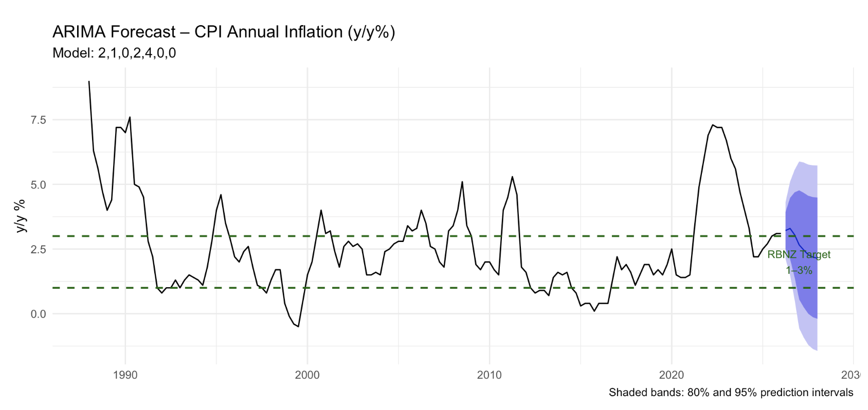
fc <- forecast(arima_fit, h = 8, level = c(80, 95))

autoplot(fc) +
  geom_hline(yintercept = c(1, 3), linetype = "dashed", color = "darkgreen", linewidth = 0.8) +
  annotate("text", x = time(cpi_ts)[length(cpi_ts)] + 1,
           y = 2, label = "RBNZ Target\n1–3%", color = "darkgreen", size = 3.5) +
  labs(title = "ARIMA Forecast – CPI Annual Inflation (y/y%)",
       subtitle = paste("Model:", arima_fit$arma %>% paste(collapse = ",")),
       x = NULL, y = "y/y %",
       caption = "Shaded bands: 80% and 95% prediction intervals") +
  theme_minimal(base_size = 13)
fc_df <- data.frame(
  Quarter   = as.character(time(fc$mean)),
  Forecast  = round(fc$mean, 2),
  Lower_80  = round(fc$lower[, 1], 2),
  Upper_80  = round(fc$upper[, 1], 2),
  Lower_95  = round(fc$lower[, 2], 2),
  Upper_95  = round(fc$upper[, 2], 2)
)
kable(fc_df, caption = "8-Quarter CPI Inflation Forecast (y/y %)")| Quarter | Forecast | Lower_80 | Upper_80 | Lower_95 | Upper_95 |
|---|---|---|---|---|---|
| 2026.25 | 3.21 | 2.50 | 3.93 | 2.12 | 4.31 |
| 2026.5 | 3.30 | 2.11 | 4.48 | 1.49 | 5.10 |
| 2026.75 | 3.05 | 1.41 | 4.69 | 0.54 | 5.56 |
| 2027 | 2.66 | 0.55 | 4.77 | -0.56 | 5.89 |
| 2027.25 | 2.46 | 0.25 | 4.67 | -0.92 | 5.84 |
| 2027.5 | 2.28 | 0.00 | 4.56 | -1.21 | 5.76 |
| 2027.75 | 2.19 | -0.13 | 4.51 | -1.36 | 5.74 |
| 2028 | 2.15 | -0.20 | 4.49 | -1.44 | 5.73 |
10. Multi-Series ARIMA Summary
Quick auto.arima fits across all major y/y series for comparison.
series_list <- list(
  "CPI"          = df$CPI_yy,
  "Tradable"     = df$Tradable_yy,
  "Non-Tradable" = df$NonTradable_yy,
  "Food"         = df$Food_yy,
  "Housing"      = df$Housing_yy
)

multi_results <- map_dfr(names(series_list), function(nm) {
  vals <- series_list[[nm]]
  vals <- vals[!is.na(vals)]
  ts_obj <- ts(vals, frequency = 4)
  fit <- auto.arima(ts_obj, stepwise = TRUE, approximation = TRUE)
  tibble(
    Series = nm,
    Model  = paste0("ARIMA(", paste(arimaorder(fit), collapse = ","), ")"),
    AICc   = round(fit$aicc, 2),
    RMSE   = round(sqrt(mean(residuals(fit)^2)), 4)
  )
})

kable(multi_results, caption = "Auto ARIMA Models – All Key Series")| Series | Model | AICc | RMSE |
|---|---|---|---|
| CPI | ARIMA(3,0,1,2,0,2,4) | 271.80 | 0.5304 |
| Tradable | ARIMA(2,0,1,2,0,1,4) | 286.50 | 0.8506 |
| Non-Tradable | ARIMA(2,0,0,2,0,0,4) | 113.21 | 0.3849 |
| Food | ARIMA(2,0,1,2,0,0,4) | 468.92 | 1.0505 |
| Housing | ARIMA(2,0,0,2,0,0,4) | 145.45 | 0.4436 |
11. Summary & Key Findings
recent <- tail(df, 8)
kable(recent %>%
  select(Date, CPI_yy, Tradable_yy, NonTradable_yy, Food_yy, Housing_yy) %>%
  mutate(Date = as.character(Date)),
  digits = 2,
caption = "Recent 8 Quarters – Key Inflation Metrics (y/y %)")| Date | CPI_yy | Tradable_yy | NonTradable_yy | Food_yy | Housing_yy | |
|---|---|---|---|---|---|---|
| 146 | 2024 Q2 | 3.3 | 0.3 | 5.4 | 0.2 | 4.4 |
| 147 | 2024 Q3 | 2.2 | -1.6 | 4.9 | 0.7 | 4.6 |
| 148 | 2024 Q4 | 2.2 | -1.1 | 4.5 | 1.3 | 4.3 |
| 149 | 2025 Q1 | 2.5 | 0.3 | 4.0 | 2.6 | 4.3 |
| 150 | 2025 Q2 | 2.7 | 1.2 | 3.7 | 4.2 | 4.0 |
| 151 | 2025 Q3 | 3.0 | 2.2 | 3.5 | 4.6 | 3.5 |
| 152 | 2025 Q4 | 3.1 | 2.6 | 3.5 | 4.3 | 3.5 |
| 153 | 2026 Q1 | 3.1 | 2.5 | 3.5 | 4.0 | 3.4 |
Narrative:
- Headline CPI inflation peaked around 9% (y/y) during 2022 post-COVID supply shock.
- As of the latest quarter, CPI is at 3.1% y/y.
- Non-tradable inflation remains persistently above tradable inflation, reflecting sticky domestic cost pressures.
- The ARIMA forecast suggests inflation returning toward the RBNZ 1–3% target band over the next 2 years.
Analysis produced with R 4.6.0 | {forecast}, {tidyverse}, {tseries}